
A lower mold price can be attractive until repeated machine time, scrap, maintenance or capacity constraints make every production release more expensive. The opposite mistake is equally costly: buying a sophisticated multi-cavity tool for demand that never arrives. A break-even calculation is useful only when both options are placed on the same commercial and technical basis.
Compare the incremental fixed investment with the credible per-part cost difference: break-even quantity equals the fixed-cost difference divided by the unit-cost difference. Then test that crossover against program demand, ramp timing, tool life, validation, cash timing and capacity. It is a screening decision, not proof that either mold will produce an approved automotive part.
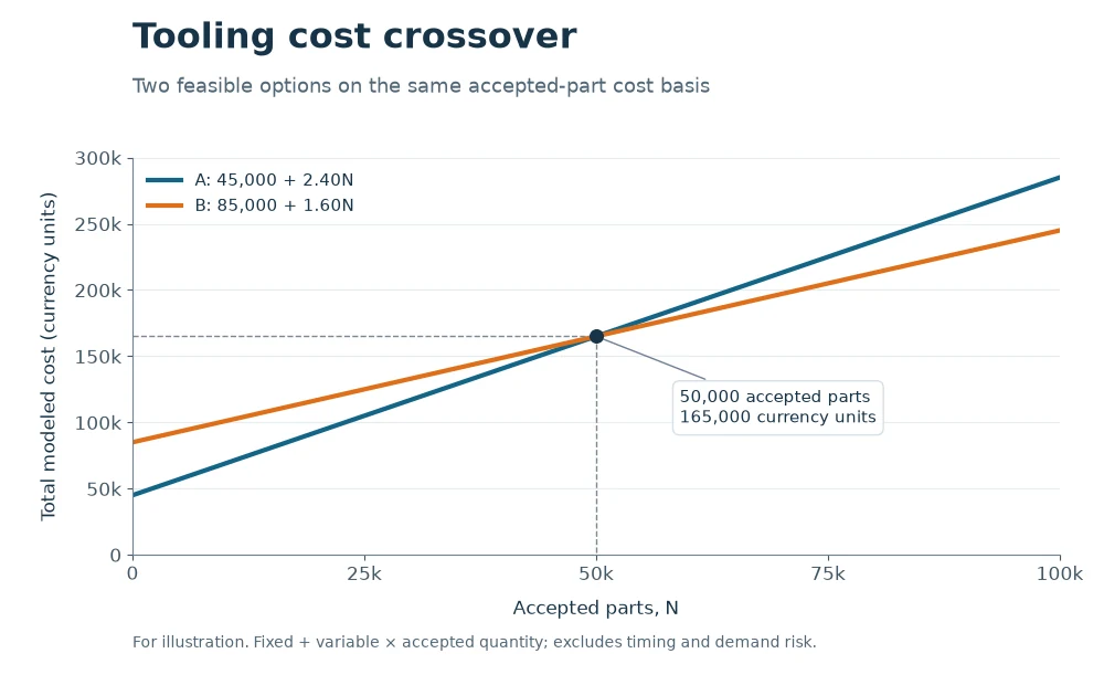
For illustration: total-cost comparison using the worked-example assumptions.
The illustration compares total cost at each accepted quantity: fixed cost + variable cost × quantity. With positive variable costs, both lines rise; their intersection marks equal modeled total cost.
Define the two options before calculating
A crossover is meaningless when one quote includes production tooling, fixtures and sampling while the other excludes them. The comparison must describe two complete and feasible routes to the same released part.
Freeze part revision, resin, annual volume, order pattern, machine class, cavity output, quality scope, packaging and delivery basis. Build an option sheet that identifies every fixed and variable item and marks exclusions. Do not compare a bridge tool against a production tool as if only mold steel differs.
Option A might use fewer cavities and a simpler runner; option B might add cavities, automation or a hot runner. State what actually creates the unit-cost delta: cycle time per saleable part, runner consumption, labor, inspection, scrap allowance, energy, maintenance or secondary operations. Keep tool payment, design, fixtures and validation in fixed cost unless the contract charges them by part. Keep resin, machine conversion and routine handling in variable cost. The tooling amortization guide explains why embedding the same tool cost in both numerator and unit price would double count it.
Build the review around aligned quotation scopes, technical assumptions and a fixed-versus-variable cost ledger. The decision is whether both options deliver the same released product and their cost differences are assigned once. Adding detail improves comparability, but false precision is worse than a visible range; use bounded inputs where suppliers cannot yet support one value.
Calculate the static crossover correctly
The basic arithmetic is simple, but signs, units and zero or negative savings often expose an invalid comparison.
For two feasible options, use N* = (Fixed B − Fixed A) / (Variable A − Variable B). Use the same currency, tax treatment, delivery point and per-saleable-part basis. If option B does not have a lower variable cost, there is no positive cost crossover under this model.
Suppose option A requires 45,000 currency units of fixed work and has a variable cost of 2.40 per accepted part. Option B requires 85,000 and has a variable cost of 1.60. The incremental investment is 40,000 and the variable saving is 0.80, so the static crossover is 50,000 accepted parts. At exactly that quantity, modeled totals are equal. This does not mean the program should automatically choose B: the calculation excludes cash timing, demand uncertainty and consequences of missing capacity. The result should be shown with its inputs and not rounded into a universal rule.
The working record should contain the calculation formula, units, source values and an independent arithmetic check rather than a conclusion copied into email. Review the source, revision, units, sample selection and boundary conditions, then test whether the crossover uses incremental fixed cost and credible variable cost per accepted part on one basis. A static model is transparent and useful for screening, while discounted cash flow or probabilistic demand models may be needed when timing and uncertainty materially affect the decision.
Use saleable output rather than theoretical shots
Cavity count and cycle time do not directly equal delivered pieces. Runner scrap, downtime, cavity imbalance and inspection holds can change the effective unit cost.
Convert each option into saleable parts per productive hour using validated or explicitly estimated cycle, active cavities, yield and planned uptime. Preserve the assumptions separately so purchasing can see which inputs are measured and which still require trial evidence.
A four-cavity tool running twice the cycle of a one-cavity tool does not automatically produce four times the accepted output. Include planned maintenance, color changes, insert loading, start-up holds,
. multi-color campaign guide explains how to schedule those color changes when several colors share one mold. If one cavity can be blocked, do not assume the original process and approval remain valid. Capacity should also be compared with peak releases, not only annual averages. The single-, multi- and family-mold comparison provides the cavity investment context; this calculation converts the chosen configurations into comparable saleable economics.
Ask the supplier to connect cycle basis, active cavity map, yield definition, downtime assumptions and capacity calculation to the proposed part and production state. The evidence is sufficient only when the variable-cost estimate represents accepted output under a supportable production pattern. Conservative yield and downtime protect the business case, but overly pessimistic allowances can hide the value of a capable production design; ranges make the sensitivity visible.
Test demand uncertainty and timing
One lifetime-volume forecast can make a fragile business case look certain. Automotive ramps, engineering changes and end-of-production timing rarely follow a straight line.
Evaluate at least low, expected and high demand cases, with release timing by year or quarter. Show where each case sits relative to break-even and whether the tool can deliver peak requirements before the modeled savings are realized.
A program may exceed the lifetime crossover but still favor the lower-investment option if most volume arrives after a design change or if capital is constrained early. Conversely, the high-investment tool may be necessary below the cost crossover when the simple option cannot meet peak weekly demand. Add ramp scrap, bank-build requirements and planned service quantities where they are part of the controlled forecast. Keep customer forecast, supplier capacity reservation and purchasing commitment distinct. The forecast and release-order guide helps separate planning signals from authorized orders.
Use time-phased demand scenarios, peak release requirements and the source and status of each forecast to challenge the preferred option. The release test is whether the preferred option remains feasible across the demand range or has a defined trigger for changing strategy. Buying flexibility costs money, while committing early can lower unit cost; the decision should value the specific option to expand, duplicate or retire the tool rather than assume flexibility is free.
Add validation, change and failure exposure
A cost model that stops at mold and machine price can select an option that is expensive to qualify, repair or change.
Include fixed and variable consequences of sampling, gauges, PPAP or customer submissions, duplicate-tool correlation, spare inserts, planned maintenance and likely engineering-change routes. Keep unsupported failure costs as scenarios rather than facts.
Higher cavity count can require more cavity-specific dimensional evidence and a broader capability study. A hot runner can reduce runner mass yet add controller, spare-tip and color-change considerations. Hardened inserts may raise initial cost but support defined wear zones; they do not guarantee tool life. A simple tool can be easier to modify but may create capacity dependence. Ask what is included at first approval and what will be charged after a change. Model only differences between options. Common validation work belongs in the baseline, not the incremental numerator.
Before closing this point, reconcile validation deliverable lists, change assumptions, maintenance scope and supplier-supported recovery scenarios with the controlled product definition. The reviewer should be able to show that the comparison includes material option-specific costs and does not turn unsupported risks into precise expected values. Including every remote event can paralyze the analysis; focus on credible mechanisms, show ranges and assign contingency separately from the base quotation.
Turn the result into a gated sourcing decision
A spreadsheet can identify a preferred option but cannot release steel, approve a process or authorize a commercial commitment.
Document the selected option, approved inputs, sensitivity limits and trigger points. Tie the decision to DFM, tool specification, machine compatibility, validation plan and commercial approval before purchase-order release.
Record what would reverse the choice: demand falling below a threshold, cycle evidence missing target, a cavity layout failing DFM, a resin change, destination-machine constraints or a customer validation change. Assign owners and dates for open inputs. If a quote is conditional, preserve the condition in the purchase baseline. At tool design release, confirm that the cost model still describes the actual mold. After trial, replace estimated cycle, yield and maintenance inputs with evidence and refresh the model before production sourcing is locked.
Release from this stage should cite signed calculation revision, sensitivity table, open-item owners and links to engineering and commercial approvals and explain why the selected option is both economically preferred and technically releasable under the current baseline. A gate may delay commitment briefly, but it prevents the organization from treating a preliminary crossover as approval for an unverified mold concept.
Break-even calculation worksheet
Use one row per controlled input. Keep point estimates and ranges visible, and calculate the crossover only after the two options use the same scope.
| Review line | Input or evidence | Decision or action |
|---|---|---|
| Fixed-cost delta | Tool, design, fixtures, option-specific validation and launch work | Subtract option A from option B once |
| Variable-cost delta | Material, machine conversion, labor, scrap, inspection and secondary work per accepted part | Subtract B from A; confirm the saving is positive |
| Static crossover | Fixed delta divided by variable saving | Compare with low, expected and high lifetime demand |
| Capacity | Saleable parts per productive hour and peak release | Reject an option that cannot meet the required window |
| Timing | Time-phased demand and payment milestones | Escalate to cash-flow analysis when timing matters |
| Triggers | Volume, cycle, yield, design and approval boundaries | Recalculate when a trigger changes |
Do not conceal uncertainty by averaging supplier ranges. Calculate the low and high crossover produced by credible input combinations, then show which input drives the decision most strongly. A buyer can then request evidence for the sensitive variables before paying for complexity.
Applying the method to a defined situation
A buyer compares a two-cavity cold-runner tool with a four-cavity hot-runner tool for the same bracket. The larger tool has a higher fixed cost and a lower modeled unit cost, but its advantage depends heavily on cycle time and saleable yield. The team calculates the static crossover, then tests it against a low-volume case, the expected program forecast and peak weekly releases. The expected lifetime volume exceeds the crossover, yet the four-cavity option is not released until machine compatibility, cavity-level sampling and hot-runner maintenance responsibilities are confirmed. If trial output misses the modeled range, the calculation is revised instead of defending the original selection.
This illustrative scenario is not a customer case.
Questions for the supplier review
- Which cost items differ between the two options, and are any counted twice?
- Is unit cost stated per shot or per accepted part?
- What measured evidence supports cycle, yield and productive uptime?
- Can each option meet peak releases and planned service demand?
- Which validation, maintenance and engineering-change costs are option-specific?
- What volume or technical trigger requires the decision to be recalculated?
Information to submit for a project-specific review
Provide the two tooling concepts or quotations, fixed-cost scope, unit-cost build-up, resin and runner basis, cavity count, cycle assumption, forecast by period, peak demand and validation requirements. Submit these inputs through the AutoMoldingPro request form. Mark unresolved points as assumptions so they can be priced and closed before tooling or production commitment.
Conclusion
Use break-even volume to expose the economic crossover, then challenge it with saleable output, demand timing, tool limits and approval costs. Release the option only when the same controlled inputs support both the calculation and the manufacturing plan.