
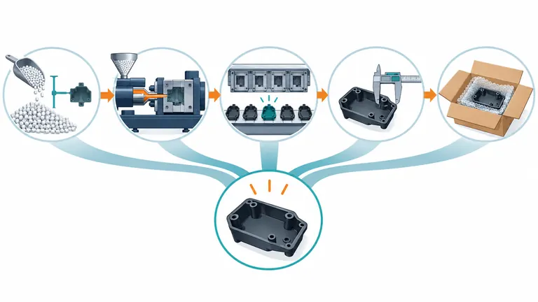
Conceptual illustration; not to scale.
An automotive molded-part price can look simple as a number per piece, yet two quotations may be based on different shot weights, cavity assumptions, uptime, scrap, inspection, packaging, and secondary operations. If those assumptions stay hidden, the lowest unit price may represent a narrower scope or an output rate the mold cannot sustain.
A defensible price is built from material consumed per acceptable part, effective machine output, labor and overhead tied to the production cell, inspection and downstream work, packaging, and agreed commercial allowances. Normalize each quote to the same resin, good-part quantity, cavity state, validated cycle, quality scope, and delivery condition before comparing the number.
Use this guide when you need to understand why a piece price is what it is. This guide explains the drivers — material, cycle time, inspection, and downstream work — and how to normalize them so quotes can be compared. It does not compare quotes for you: for the comparison matrix and the low-quote screen, use How to Compare Automotive Injection Molding Quotes Beyond Mold Price. And it does not give the total cost of a part delivered from China: packaging, freight, duty, and carrying cost are landed-cost items, and the per-accepted-part total is built in Total Landed Cost of Automotive Molded Parts from China: A Buyer’s Calculation Checklist. Use the driver sheet in this guide to make quotes comparable, the comparison matrix in 250 to rank them, and the landed-cost checklist in 388 to judge the delivered total.
Build the model around one acceptable shipped part
Start by defining the unit being priced. Is it one loose molded component, one cavity-identified component, one assembled set, or one packed unit? Does the price include runner material, inserts, labels, inspection reports, protective packaging, export cartons, freight, duty, tooling amortization, or launch costs? A quote cannot be compared until the commercial unit and boundary are the same.
A useful recurring-cost model is:
unit price = material per good part + conversion per good part + direct downstream work + packaging + agreed overhead and margin
This is a framework, not a universal accounting rule. Suppliers allocate labor, utilities, overhead, depreciation, maintenance, and margin differently. The buyer’s objective is to expose the physical drivers behind the quoted result. Machine conversion is commonly related to an hourly cell rate divided by acceptable pieces produced per hour. The denominator must use effective cavities and effective runtime, not merely the nominal cavity count and theoretical cycle.
Keep non-recurring items separate unless the commercial agreement intentionally amortizes them. How that amortization is structured — direct payment, per-part recovery, or a hybrid, over what denominator, and what happens to the piece price after recovery — is decided in Automotive Tooling Amortization: Separating Mold Investment from Part Price; this guide prices the recurring part, it does not choose the recovery model. Mold manufacture, gauges, fixtures, validation testing, PPAP preparation, special sampling, and engineering changes may be quoted as one-time charges or spread across a committed volume. If amortization is used, record the volume, start and end conditions, ownership, treatment of early program termination, and whether the unit price changes after recovery. Otherwise, tooling can be counted once in the purchase order and again inside the piece price.
Define acceptable output with the customer’s current drawing, appearance standard, material, and control plan. A part that is dimensionally acceptable but fails assembly, cleanliness, identification, or packaging criteria is not an acceptable shipped part. This boundary prevents a low conversion estimate from hiding downstream sorting or rework.
Material cost begins with the shot, not only the CAD weight
The finished-part mass is only one part of material consumption. A cold-runner mold also produces sprue and runner mass per shot. Startup, purge, color change, sampling, retention samples, process stabilization, and rejected pieces consume additional material. Inserts and purchased components may add their own unit cost and incoming-loss assumptions. The RFQ should therefore identify finished mass, runner strategy, expected regrind policy, resin grade, color or additive system, and who supplies each material.
Calculate physical material use at shot level. For an illustrative four-cavity tool, the gross shot contains four molded parts plus the runner. Divide gross material by four only when all four cavities produce acceptable parts. If one cavity is disabled, the shot may still consume nearly the same runner and three part charges while yielding only three pieces. The material and conversion denominators both change. Do not treat the disabled cavity merely as a scrap-rate adjustment if the quoted cycle and runner remain unchanged; that can double-count or misstate the loss.
Regrind should not be assumed to have zero cost or universal approval. Its use depends on the resin, color, contamination controls, drying history, mechanical requirements, appearance, regulatory or customer restrictions, and the approved process. If regrind is permitted, state the source, maximum proportion, handling, traceability, and how property risk is controlled. If it is not permitted, runner and purge material become a clearer direct cost.
Use the exact commercial resin grade and applicable condition. Material manufacturers publish grade-specific processing and property data; those data do not automatically transfer to another grade or recycled-content variant. Resin price also changes with purchase quantity, supply terms, color package, drying and storage burden, and yield. Ask suppliers to separate the resin price basis from the consumption factor so that market changes do not obscure an engineering difference.
Cycle time must be converted into effective good-part output
The theoretical output of a mold is straightforward: 3600 seconds ÷ cycle seconds × nominal cavities. The commercial output is lower whenever the cell is not running, cavities are unavailable, or parts are rejected. A more useful denominator is theoretical pieces × runtime factor × good-part yield, with each factor defined from non-overlapping losses.
RJG’s official injection-molding ROI calculator treats parts per cycle, cycle time, uptime, scrap rate, machine rate, labor, part weight, and runner weight as separate inputs. That separation is valuable because it prevents the same downtime or scrap from appearing in several factors. A supplier may use a different costing system, but it should be able to reconcile equivalent physical assumptions.
Ask whether the quoted cycle is simulated, estimated from a similar part, observed during a short trial, or demonstrated during a production-intent run. Cooling, mold opening, ejection, robot removal, insert loading, in-cycle inspection, and safe handling all affect the cycle. Husky’s hot-runner fundamentals explain why a cold runner can add cooling and handling time, but a hot runner is not automatically the best economic choice; it adds tooling, control, maintenance, and changeover considerations.
Record the effective cavity assumption. Multi-cavity balance matters because the process window must protect the first cavity that flashes and the last cavity that fills. Husky notes that cavity balance influences the usable process window and qualification. A quotation based on eight sellable parts per shot is not equivalent to one that has priced a contingency for a blocked cavity or cavity-specific inspection.
Finally, define the cell rate boundary. It may include the press, robot, dryer, temperature controller, operator, maintenance allocation, floor space, utilities, and normal overhead. Do not add separate labor again if it is already included in the cell rate. Ask for the boundary rather than demanding confidential accounting detail.
Inspection and downstream work can govern the unit price
Inspection cost is driven by what is checked, how often, with which method, and what evidence must be retained. “Standard inspection included” is not a measurable scope. Identify receiving checks on resin and inserts, startup approval, cavity-specific dimensional checks, appearance inspection, gauge use, destructive testing, functional assembly, periodic capability studies, final audit, record retention, and customer submission work.
Measurement frequency alone is not enough. A manual fixture check may take seconds, while a CMM layout, contour scan, electrical test, cleanliness analysis, or conditioned dimensional study requires different equipment, setup, and reporting. If the drawing contains critical characteristics, agree how those characteristics flow into the control plan and whether the measurement system is suitable. AIAG identifies MSA and SPC as part of the connected quality core tools; using the names does not define the customer’s exact sampling plan, acceptance criteria, or submission level.
Downstream operations often create the real constraint. Degating, deflashing, insert loading, pad printing, laser marking, welding, assembly, leak testing, cleaning, and protective packaging can require labor, fixtures, consumables, maintenance, and yield allowances. State whether the quoted piece price includes these steps and whether their yield is combined with molding yield or calculated separately. Combining is acceptable if it is transparent; applying both an overall scrap allowance and separate operation losses without reconciliation is not.
Packaging should match part risk. Cosmetic surfaces may require non-contact pockets. Long thin components may need support against creep or distortion. Electrical parts may need cleanliness, closure protection, or customer-specific labels. Export cartons, pallets, returnable totes, and dunnage change both unit cost and logistics. Price the approved pack quantity and replacement responsibility, not a generic bag-and-box assumption.
Normalize quotations with a driver sheet
Use one comparison sheet and ask each supplier to confirm or correct the assumptions. The purpose is not to force identical accounting. It is to make differences explainable.
| Driver | Common comparison basis | Evidence or clarification |
|---|---|---|
| Commercial unit | One acceptable packed part or defined assembly | Scope statement and packaging specification |
| Resin | Exact grade, color, supplier responsibility and price date | TDS, quotation basis, material certificate plan |
| Material use | Part mass, runner mass, purge/startup and approved regrind | Shot calculation and runner layout |
| Mold output | Nominal and effective cavities | Cavity map and balance/maintenance assumption |
| Cycle | Production-intent cycle and included operations | Trial record or clearly marked estimate |
| Runtime and yield | Non-overlapping uptime and scrap factors | Capacity model and historical/assumed basis |
| Inspection | Characteristics, frequency, method and reports | Draft control plan and inspection scope |
| Secondary work | Operation, fixture, labor, consumables and yield | Process flow and responsibility matrix |
| Packaging/logistics | Pack quantity, dunnage, labels and delivery term | Packaging proposal and Incoterm |
Illustrative example: Supplier X quotes a lower machine rate but assumes a six-cavity tool, a shorter unverified cycle, standard visual inspection, and bulk packaging. Supplier Y assumes four effective cavities, includes cavity-specific checks on two interfaces, and uses partitioned trays. The prices cannot be ranked until the buyer decides which mold concept, evidence scope, and packaging are required. The exercise may reveal that neither quote is “wrong”; they answer different questions.
Worked example — one acceptable part, fully calculated (illustrative)
Illustrative example — hypothetical teaching numbers, not an AutoMoldingPro quotation and not a real supplier price. Every input below is assumed for the purpose of showing the arithmetic; substitute the actual part, resin grade, cycle, cell rate, and inspection scope before using this method on a real quote. No percentage, saving, or cost figure in this example is taken from any other supplier’s page.
Assumed inputs (all stated, none hidden): four-cavity tool, all four cavities effective; production-intent cycle 30 seconds; runtime factor 0.85; good-part yield 0.97; cell rate USD 90 per hour (press, robot, dryer, operator, and normal overhead — one boundary, counted once); molded part mass 40 g; cold-runner mass 16 g per shot; resin USD 3.00 per kg; downstream work (degating and protective packing labour) USD 0.05 per good part; packaging USD 0.04 per good part; agreed overhead and margin allowance USD 0.05 per good part.
Step 1 — effective good-part output. Theoretical output is 3,600 ÷ 30 × 4 = 480 parts per hour. Effective good-part output is 480 × 0.85 × 0.97 = 395.76, rounded to 396 good parts per hour. The denominator uses effective cavities and effective runtime, not the nominal cavity count and theoretical cycle, as the model in "Build the model around one acceptable shipped part" requires.
Step 2 — conversion per good part. USD 90 per hour ÷ 396 good parts per hour = USD 0.23 per good part.
Step 3 — material per good part. Gross shot mass is (4 × 40 g) + 16 g = 176 g, or 44 g per molded part. At USD 3.00 per kg that is USD 0.132 per molded part. Divided by the good-part yield of 0.97, material is USD 0.14 per good part (USD 0.136 unrounded). The runner is charged to the part because this is a cold-runner tool; regrind is assumed not permitted here, so runner and purge material stay a direct cost.
Step 4 — add the remaining lines and total.
| Cost line | Per good part (USD) |
|---|---|
| Material per good part | 0.14 |
| Conversion per good part | 0.23 |
| Direct downstream work | 0.05 |
| Packaging | 0.04 |
| Agreed overhead and margin | 0.05 |
| Total unit price, one acceptable shipped part | 0.50 |
Unrounded total is USD 0.503, shown as USD 0.50. If any assumed input changes, the total changes with it — that is the point: the buyer can now ask Supplier X which input differs (the unverified cycle, the six-cavity assumption, the inspection scope, or the packaging) instead of arguing about the final number.
Sensitivity — one cavity blocked. If one cavity is disabled and the shot still consumes nearly the same runner, theoretical output falls to 3,600 ÷ 30 × 3 = 360 parts per hour and effective good-part output to 360 × 0.85 × 0.97 = 297 good parts per hour. Conversion rises to USD 90 ÷ 297 = USD 0.30 per good part, and material rises to 176 g ÷ 3 = 58.7 g per molded part, or USD 0.18 per good part after yield. The total becomes USD 0.62 per good part — about 24% higher than the four-cavity case — even though the cycle never changed. This is why the article warns against treating a disabled cavity merely as a scrap-rate adjustment: the material and conversion denominators both change.
Once current production data confirms the cost baseline, use a controlled cost-reduction plan to evaluate changes and verify the savings. That plan — the fill-in opportunity register, the saving formula per row, and the validation each change needs — is in Reducing Cost in Mature Automotive Molding Programs: Where to Start; this guide establishes the baseline the plan starts from, it does not run the cost-down program.
Before requesting a revised price, freeze the resin grade, part and runner mass basis, annual and peak demand, order quantity, cavity strategy, validation and inspection scope, secondary work, packaging, and delivery term. For a project-specific assessment, submit the STEP file, 2D drawing, material requirement, annual volume, and inspection expectations through the AutoMoldingPro RFQ page.