
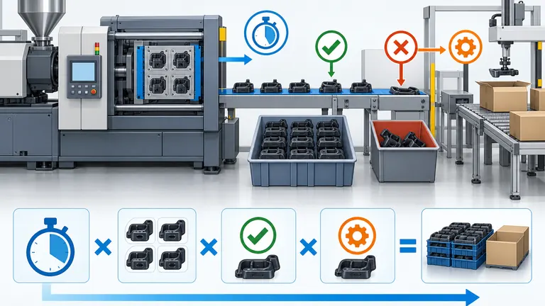
Conceptual illustration; not to scale.
Home › Blog › Automotive Molding Capacity: What a Run-at-Rate Trial Should Demonstrate
Automotive sourcing and manufacturing decision guide
A molding cell can appear fast while the delivered route remains short of demand. Nominal cycle time ignores startup, downtime, disabled cavities, rejects, inspection, assembly, and packaging. If those losses are mixed or counted twice, a Run at Rate can produce an impressive number that neither planning nor the customer can reproduce.
A defensible Run at Rate records conforming output across a defined scheduled window under intended production conditions and through the agreed delivery boundary. Reconcile scheduled time, running time, completed shots, active cavities, gross pieces, holds, rejects, and downstream accepted units. Compare that demonstrated rate with a demand model that uses the same units and applies each loss exactly once.
The decision depends on three controls: a testable capacity question, a production-representative route, and arithmetic that an independent reviewer can reproduce.
In This Guide
- Define the Capacity Question Before Starting the Clock
- Use Intended Production Conditions and Record Deviations
- Illustrative Capacity Calculation Without Double-Counting Losses
- Test the Full Route and the Real Bottleneck
- Run-at-Rate Record Points
- Make a Bounded Capacity Decision
Define the Capacity Question Before Starting the Clock
Why this matters: Capacity statements often mix annual demand, hourly machine output, calendar hours, and finished assemblies. Without one numerator, denominator, and process boundary, a pass or fail has no stable meaning.
Define the required good delivered units per scheduled hour and the demand period it must support. State whether the boundary ends at molding, inspection, packaging, or assembly, and identify the customer-specific form, duration, witnessing, and pass rule before the run.
State the required good-piece rate, demand time basis, shift pattern, launch/steady-state condition, number of tools and lines, planned maintenance, changeovers and downstream operations. “Can make 500,000 parts per year” is not testable until the available hours and losses are defined.
Choose the boundary: molding cell only, packaged part or finished assembly. If the customer buys a labeled assembly, a fast molding press does not prove deliverable capacity when trimming, inspection, assembly or packaging is slower.
Record whether the trial is a short demonstration, significant production run, capacity verification or customer-specific Run at Rate. Those names may carry different contractual rules. Use the customer’s form when one is mandated.
Translate the commercial forecast into an engineering demand case. Begin with pieces per vehicle or finished unit, program volume by period, service demand, launch ramp, peak mix, and any agreed contingency. Then identify planned working days, shifts, scheduled hours, holidays, maintenance, changeovers, and tool sharing. Keep assumptions visible: a requirement of 500 good parts per shift is different from 500 gross molded pieces, and neither can be compared directly with an annual number until the time basis is reconciled.
Use a one-page capacity-question sheet as the working tool. Required fields are part and revision, good-unit requirement, period, shift pattern, process start and end points, tools and active cavities, downstream steps, scheduled trial window, required records, witness, and decision authority. Illustrative use scenario: a buyer needs 960 packaged clips in one eight-hour shift. The molding cell target cannot simply be 120 pieces per hour because planned changeover, inspection holds, and pack-station breaks may fall inside that shift. The team must agree whether the trial includes those losses or models them separately before the clock starts.
Demand numerator
Good parts or finished assemblies required, including the defined service/contingency treatment—never an unlabeled gross shot count.
Time denominator
Scheduled hours, net running hours or calendar hours. Name which losses are already removed.
Process boundary
Tool/press/cavities plus every required downstream operation, inspection and packaging step.
Use Intended Production Conditions and Record Deviations
Why this matters: A demonstration made with temporary labor, a different press, hand sorting, or an unapproved material can generate useful learning but does not prove that the intended serial route will deliver the same rate.
Run the intended production tool, equipment, material, staffing, process, inspection, and packaging wherever possible. Record every substitute or temporary control, explain the remaining risk, and set a separate closure action instead of treating the deviation as serial evidence.
AIAG’s PPAP errata states that a Production Demonstration Run or Run at Rate may be required by certain customers before the Part Submission Warrant; it is not a universal duration or sample-count rule. Volvo Group’s public supplier quality manual likewise says its Supplier Quality Engineer and supplier define how many parts to produce and when to perform the run.
Volvo’s significant production run guidance calls for production tooling and equipment, the production environment and operators, and the production cycle time; it also says the run should support process stabilization, throughput, capacity and capability assessment.
Record tool and cavity IDs, press, robot, dryer, temperature controller, material grade/color/lot, regrind rule, staffing, inspection resources, packaging, shift and software/program revisions. If a prototype fixture, extra operator or off-line inspection is used, label the deviation and assess whether the serial route can reproduce the result.
Do not pre-delete downtime to make the rate look stable. Classify each stop: planned break, material interruption, tool/press alarm, quality hold, adjustment, inspection wait, downstream blockage or other. The record should show whether the trial observed the loss or whether planning applies a separately agreed factor.
Prepare a condition-comparison sheet before the run. One column states the intended serial condition and a second states the trial condition for press, clamp and shot capacity, robot, dryer and material feed, temperature control, cavity status, resin and color, regrind policy, process program, operators, gauges, fixtures, secondary operations, labels, and packaging. Classify each difference as equivalent with evidence, more favorable than serial, less favorable than serial, or not assessed. A favorable temporary condition—such as an extra inspector—still creates an open production risk because the future line will not have that resource.
Verify readiness at the line rather than from documents alone. Confirm identifiers, calibration or verification status where required, approved work instructions, material traceability, inspection availability, packaging supply, and data collection clocks. Define stabilization and sampling start so setup scrap is visible but not confused with accepted output. During the run, avoid unplanned process adjustment unless the event and its impact are recorded. A Run at Rate is not a contest to protect a target number; an alarm, quality hold, blocked chute, or operator intervention is evidence about the route that planning needs.
Illustrative Capacity Calculation Without Double-Counting Losses
Why this matters: Capacity calculations fail when observed downtime and rejects are embedded in an output rate and then deducted again, or when a theoretical cycle is multiplied by optimistic availability and yield factors with no evidence.
Use either an observed scheduled-window rate or a clearly separated elemental model, then reconcile the two. Maintain shot, piece, quality-status, and time balances so cavities, losses, and units are visible and each factor is applied once.
Illustrative example — assumptions: two-cavity mold; observed stable cycle 42 seconds/shot; scheduled trial window 180 minutes; 30 minutes of recorded downtime; 214 completed shots during 150 running minutes; 428 gross pieces; 17 rejected pieces; 411 good pieces.
Observed net-running check: 150 min × 60 sec/min ÷ 42 sec/shot = 214.3 theoretical shots, consistent with 214 completed shots after whole-shot rounding.
Observed good rate across the scheduled window: 411 good pieces ÷ 3.0 scheduled hours = 137 good pieces/hour. This rate already contains the observed downtime and rejects. Do not multiply it by uptime or yield again.
Elemental planning alternative: theoretical gross rate = 3,600 sec/hour ÷ 42 sec/shot × 2 cavities = 171.4 pieces/hour. If a separate annual model assumes 3,600 scheduled hours, 85% uptime and 96% good yield, planned annual good output = 171.4 × 3,600 × 0.85 × 0.96 ≈ 503,500 pieces/year. Here uptime and yield are each applied once.
The observed and elemental methods answer different questions. Use the observed all-window rate when the trial window is representative. Use an elemental model for scenario planning, but substantiate each factor and reconcile it to actual data.
Put the calculation in a locked worksheet with labelled inputs and units. The observed route should show scheduled minutes, downtime by reason, net running minutes, completed shots, active cavities by interval, gross pieces, setup pieces, rejects, held pieces, and released good pieces. If a cavity is disabled mid-run, split the interval rather than multiplying every shot by the nominal cavity count. If held pieces are later released, update the disposition without changing the original production event. Preserve raw counters or machine reports beside the summarized sheet.
Use the illustrative numbers to test the worksheet logic. The 137-good-pieces-per-scheduled-hour result already includes the recorded 30 minutes of downtime and 17 rejects, so applying 85% uptime and 96% yield to 137 would understate the same run twice. Conversely, the 171.4 gross pieces per running hour contains neither loss and therefore needs explicit planning factors. Ask what evidence supports each annual-model factor, how maintenance and changeover are handled, and whether demand uses pieces, kits, or assemblies before approving the extrapolation.
| Calculation step | Assumption and result |
|---|---|
| Shot balance | Completed shots × active cavities = gross pieces. Reconcile short shots, purges, setup pieces and cavity-off conditions separately. |
| Good-piece balance | Gross pieces − nonconforming/held pieces = released good pieces. Define when held parts become good or reject. |
| Time balance | Scheduled window = net running time + all recorded stop categories. Do not remove a stop and also apply it as an uptime loss. |
Test the Full Route and the Real Bottleneck
Why this matters: The press may exceed target while a slower inspection, assembly, labeling, or packaging step controls shipment output. Shared equipment can also be available for the trial but unavailable in the normal product mix.
Measure accepted flow through the entire agreed route and report the slowest sustainable constraint. Record queues, staffing, fixture quantity, rejects, changeovers, and shared-resource loading; do not claim finished-part capacity from the molding rate alone.
Measure molding, degating, trimming, insert loading, inspection, assembly, labeling and packaging rates. Include fixture quantity, operator cycle, changeover, queue and reject/repair loops.
Illustrative example — continuation: the molding cell delivers 137 good pieces/hour across the observed window, but a required inspection-and-pack station sustains only 120 accepted pieces/hour with the intended staffing. The demonstrated route rate is no more than 120 packaged pieces/hour until the downstream constraint changes and is re-evaluated.
Check shared resources. A dryer, crane, CMM, leak tester or assembly fixture may be available during one trial but simultaneously required by other products in normal production. Capacity evidence should state dedicated versus shared loading and any assumed schedule separation.
Draw a simple route map and give each step an input count, accepted output count, active time, waiting time, staffing level, and reason for loss. A downstream step with a short manual cycle may still constrain the line through batch inspection, fixture cooling, label replenishment, or quality release delays. Look for accumulated work in process: a growing queue before one operation is practical evidence that its effective throughput is below the upstream rate. Also confirm whether rejected downstream parts require remolding, because that demand feeds back into the required molding output.
Illustrative decision: the molding cell produces 137 good pieces per scheduled hour, but the intended inspection-and-pack station sustains 120 accepted pieces per hour. The current demonstrated route is bounded at 120, even if temporary storage lets the mold continue during a short trial. The corrective options may include method improvement, another qualified fixture, revised staffing, automated inspection, or a customer-approved sampling strategy. Each option changes cost, validation, and error-detection risk; re-evaluate the affected route rather than simply replacing 120 with a planned future number.
Cell constraint
- Cycle stability by cavity
- Robot/degating cycle
- Material drying and feed
- Tool/press alarms
Quality constraint
- Inspection cycle and sampling
- Gauge/CMM availability
- Hold and disposition time
- Rework/repair route
Delivery constraint
- Assembly/label rate
- Packaging replenishment
- Warehouse/lot release
- Shared labor and fixtures
Run-at-Rate Record Points
Why this matters: A single average rate cannot show whether the run used the right conditions, where time was lost, which cavities failed, or what part of the route was excluded. It is weak evidence for later planning.
Maintain a reproducible Run-at-Rate record with identity, conditions, chronological time losses, shot and piece balances, quality status, downstream output, raw evidence, open actions, and the exact decision boundary.
The record should let an independent reviewer reproduce the result and identify what was not tested.
Use the record-point table as a pre-run checklist and a post-run reconciliation tool. Before starting, complete the header and conditions sections and have the responsible functions confirm the target and boundary. During the run, capture events against one synchronized time source; include the start, stop, duration, category, affected equipment or cavity, output effect, and disposition. At completion, reconcile machine counters with container counts, quality records, held stock, scrap, and packaged units. Unexplained differences should remain open rather than being assigned to a generic loss bucket.
Attach evidence by reference, not by embedding uncontrolled screenshots into a summary. Useful records can include process traces, downtime export, material lot documents, inspection results, cavity-level reject log, operator and fixture assignments, pack counts, and witness sign-off where required. Protect the raw record from retrospective editing and issue a corrected revision if an error is found. An independent reviewer should be able to recalculate the demonstrated rate, identify excluded operations, and see which observations support every qualification in the final decision.
| Record point | Evidence to retain |
|---|---|
| Header | • Part/revision/customer • Date, shift and run purpose • Tool/cavity/press/line IDs • Required rate and time basis |
| Conditions | • Material grade/color/lot and drying • Process/program revision • Operators and standard work • Inspection/assembly/packaging setup |
| Time | • Scheduled start/stop • Net running time • Every downtime event and reason • Changeover and planned breaks treatment |
| Output | • Shots and active cavities • Gross, good, reject and held pieces • Rejects by cavity/reason • Downstream accepted output |
| Evidence | • Cycle trace and process alarms • Inspection/capability records • Material and lot trace • Witnesses and supporting files |
| Decision | • Demonstrated rate and boundary • Open constraints/actions/owners • Conditions for extrapolation • Customer approval or rerun requirement |
Make a Bounded Capacity Decision
Why this matters: One successful run is sometimes converted into an unconditional annual capacity promise. That ignores duration, product mix, seasonal demand, maintenance, changeovers, shared resources, and deviations that the trial did not exercise.
State the demonstrated good-unit rate, conditions, route boundary, and confidence limits, then compare it with the approved demand model. Release capacity only to the named scope and close or mitigate every material gap before relying on annual extrapolation.
Report “demonstrated under these conditions,” rather than converting one trial into an unconditional annual-capacity claim. Identify the confidence boundary: trial duration, demand mix, planned downtime, cavity condition, shared resource loading and any manual work not exercised.
Ford’s public supplier-quality page lists ePPAP, measurement-system analysis and online quality training as separate resources. That is a useful signal to keep capacity evidence, measurement controls and customer submission requirements connected but not conflated.
For a supplier-specific production review, compare the run boundary with the automotive plastic injection molding process and the evidence plan on the quality and automotive validation page. Use the project RFQ to state the required good-piece rate and downstream scope.
Scope boundary: This article is a planning aid, not an OEM approval rule. The released drawing, contract, customer-specific requirements and agreed validation plan control the actual project.
Use a bounded decision statement: “Under revision X, tool and cavities Y, line Z, stated staffing, and the observed three-hour scheduled window, the route produced N accepted packaged units per hour; the following conditions were not demonstrated.” Follow it with the required rate, calculated margin on the same basis, open risks, action owner, due date, and trigger for rerun. Avoid universal margin thresholds. The customer, product risk, demand volatility, maintenance strategy, and alternative capacity determine what reserve is acceptable.
Then test scenarios outside the trial: launch peak, service orders, another product using the same press or gauge, planned tool maintenance, cavity loss, material changeover, weekend staffing, and downstream downtime. Do not add every conservative factor simultaneously if it represents the same loss. If the decision depends on a second tool, approved overflow source, or future automation, identify that dependency and its readiness evidence. Capacity approval should be revisited after meaningful tool, process, material, routing, staffing, or demand changes under the applicable customer rules.
Conclusion
Define required good output, scheduled time, and the complete delivery route before the trial. Reconcile time, shots, cavities, quality status, and downstream units, then issue a bounded capacity decision. For review, provide demand by period, shift assumptions, tool and cavity plan, route map, intended conditions, and customer-specific Run-at-Rate requirements.
Related Decision Guides
- Planning a Pilot Production Run for Automotive Plastic Parts
- T1 Sample Approval vs. Production Release: What Still Needs to Be Closed?
- Keeping Repeat Automotive Molding Orders Consistent with Approved Samples
Define the Rate, Time Basis and Process Boundary
Provide annual demand, peak pattern, tool/cavity plan, required downstream operations and customer-specific run requirements. Capacity can then be evaluated in good delivered units, not nominal shots.
If the inquiry popup does not open in your browser, use the full automotive project RFQ.